Ranking Stocks Like Google Ranks Pages: A Learn-to-Rank Backtest of the S&P 500
Having recently received my CFA designation, I’m sharing the results of a side project I took on while awaiting my final exam results — a chance to bridge my engineering background with the CFA curriculum.
Disclaimer: this is a personal educational side project using publicly collected data, not investment advice.
The goal was to develop a Learn-to-Rank (LTR) stock-picking algorithm with a slim feature set and backtest its performance against SPY using recent market data.
Why Learn-to-Rank (LTR)?
While typically associated with search engines and recommendation systems, LTR models have a powerful use case in systematic trading. Unlike traditional z-score models that assume linear relationships, LTR can learn complex, non-linear interactions between features, making them advantageous in the domain of finance where complex non-linear relationships tend to exist between explanatory variables in predicting stock returns.
For this project, I utilized Python and the XGBoost library, specifically leveraging a pairwise ranking objective. Instead of predicting an absolute return, the model learns the relative preference between pairs of stocks—somewhat mimicking the decision-making process of a Portfolio Manager.
The Model Architecture
I utilized the S&P 500 as my universe, training the model on three core features to rank stocks for monthly rebalancing:
- 12-Month Cumulative Return: A classic momentum indicator.
- Distance from 200-Day Moving Average: Used here as a secondary momentum signal for trend confirmation. Crucially, the model can also learn to identify trends that have “overshot,” potentially signaling mean reversion when the distance becomes extreme.
- Idiosyncratic Volatility: By assuming returns follow a linear equation based on stock alpha and systematic risk (see footnote), I calculated the standard deviation of the residual error term over the last 256 days. This measure of “unaccounted for” risk adds a vital counter-weight to prevent the model from over-leveraging on pure momentum during high-uncertainty periods.
Data Preparation & Preprocessing
Because I was constrained to publicly available data—effectively taking features based on fundamental data off the table—I collected monthly close data for all tickers in the S&P 500 from 2000–2024 (inclusive). To ensure the model was training on “clean” signals, I applied three preprocessing techniques:
- Logarithmic Transformation: Applied to the idiosyncratic volatility data to normalise its distribution (it is assumed to be log-normally distributed) and improve model convergence.
- Winsorization: To limit the influence of extreme outliers in the returns data.
- Standardization: To bring all features onto a comparable scale, ensuring the XGBoost model wasn’t biased toward features with larger raw numerical ranges.
Model Training
Each monthly group of tickers with their features and their rankings for subsequent-month returns was used as a “query” in the XGBoost training set, with the goal of predicting the most accurate ranking of the 500 stocks for each query in the test data set.
After splitting the data and completing the training, the model produced an NDCG@25 of approximately 0.10 on the test data. To contextualise that number, I compared against a random-ranking baseline — a Monte Carlo over the test queries using a binary relevance encoding (top-25 = 1, rest = 0) — which yielded an NDCG@25 of approximately 0.05. The model therefore beats random by roughly 2×, indicating a real, if modest, signal in prioritising the “head” of the distribution — the part of the ranking that actually matters for a top-25 portfolio.
Simulation & Results
To simulate institutional conditions (somewhat), I ran the backtest with $1 Billion starting capital and applied 10bps transaction costs to portfolio turnover — a conservative all-in estimate for monthly rebalancing in large-cap S&P names at this AUM, covering commissions, half-spread, and modest market impact. The S&P 500 universe ensured sufficient liquidity for the $1B simulated AUM.
The model took an equally-weighted position in the top 25 stocks ranked by the trained LTR model and was rebalanced monthly. The chart below shows the simulated portfolio value over 2025 against an SPY buy-and-hold benchmark, both starting at $1B:
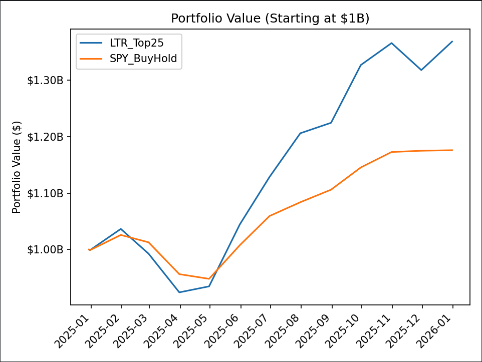
Headline 2025 results vs SPY buy-and-hold:
| Metric | LTR Top 25 | SPY Buy & Hold |
|---|---|---|
| Total Return | 36.85% | 17.60% |
| Sharpe (annualised, monthly returns) | 1.65 | 1.47 |
| Sortino (annualised, monthly returns) | 3.95 | 2.91 |
| Max Drawdown | -10.84% | -7.58% |
| Avg Drawdown | -4.82% | -3.84% |
| Avg Drawdown Days | 51.33 | 76.50 |
| Avg Up Month | 5.36% | 2.74% |
| Avg Down Month | -4.88% | -2.57% |
The strategy outperformed SPY on absolute return, on risk-adjusted return (Sharpe, Sortino), and recovered from drawdowns roughly 30% faster on average.
It also exhibited higher volatility in both directions — the average down month was nearly 2× as severe as SPY’s, and the max drawdown was meaningfully deeper. This is the expected shape of a concentrated 25-stock long-only momentum book versus a diversified 500-stock index: more upside per favourable month, more downside per unfavourable one. The faster drawdown recovery and stronger Sortino suggest the trade-off was net favourable in 2025, but the picture is more nuanced than the headline 36.85% return suggests in isolation.
This indicates that even a slim, price-driven model can potentially serve as a powerful momentum signal within a broader quantitative strategy.
Limitations
A significant critique identified in this iteration is Survivorship Bias. Because training was performed on current S&P 500 constituents (training data covered 2000–2024, with 2025 held out for testing), companies that didn’t “survive” the index were excluded. That means it was blind to the existence of Bear Stearns, Lehman Brothers, etc (yikes!). To make this production-ready would involve retraining on point-in-time data to ensure the model accounts for companies that fell out of the index over time.
A second critique is the thin out-of-sample window. A 12-month OOS period is a single data point — Sharpe and other risk-adjusted estimates over a single year carry enormous standard errors, and the strategy’s 2025 outperformance establishes that it survived one year, not that it has a stable edge. The natural next step is multi-year walk-forward evaluation across 2022, 2023, and 2024 to test whether the signal persists across different market regimes.
It’s been a rewarding challenge to apply the quantitative rigour of my engineering roots to the complex world of investment management.
Note on Idiosyncratic Volatility
The linear-regression decomposition R = α + β·Market + ε splits a stock’s return into three parts:
- α — value added (or lost) by the stock, independent of market movement.
- β — sensitivity to the market: how much the stock moves with broad market returns.
- ε — the residual: the portion of return not explained by the market.
Idiosyncratic volatility is the standard deviation of ε over the lookback window — the part of a stock’s return the market can’t account for, and the feature I used in the model.